Modeling TDCR contacts - the Kinematic way
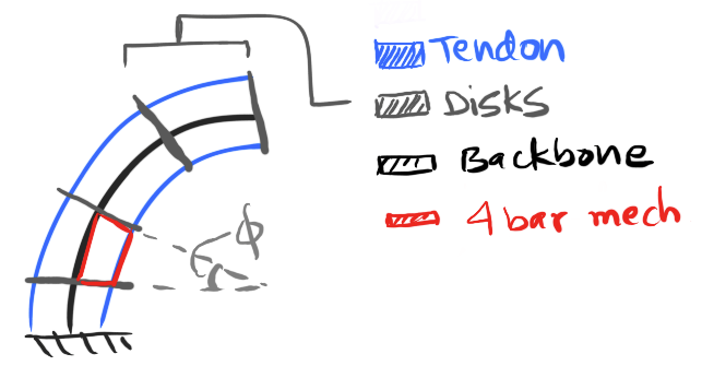
While studying different backbone representations for our survey paper [cue : shameless plug], I came across this very interesting representation where the portion of the robot between two disks (hereon referred to as a subsegment) is modeled as a series of four bar mechanisms stacked over each other. A rough sketch of one such subsegment being approximated by a 4-bar linkage (marked in red) is shown below.

While interesting in its own right, the point of this blogpost is to rewrite the proposed model using the PCCA model, introduced here - Rabbit hole to backbone representation using piecewise constant curvature arcs , to instead model contacts. The backbone is instead divided into a series of constant curvartures that each subtend an angle $\theta_j$. Do note that angles Ⲫ and θ essentially denote the same value.
Basic principle behind the forward kinematic modeling
So, forward kinematic modeling is like figuring out how something changes its shape when you pull a tendon on it or when it’s in a different environment. Imagine you’re squishing a toy robot - it will bend and change shape. But there’s a special shape it wants to be in when everything is balanced out. That’s what we call its “static equilibrium shape.” And this shape minimizes how much it’s being stretched or squished, which we call “strain energy.” [Credits to ChatGPT for that simple explanation]
Now, here comes the interesting part. In this research paper, they show that at static equilibrium, the potential energy of all the subsegments is minimized. And what this means it is ends up in a shape where the summation of θ (or Ⲫ) over all the subsegment is minimized.
Now, when we know the input tendon length thats actuating the robot, we can turn this into a math problem. We’re trying to minimize these angles as much as possible, and we also want the total length of the tendon to match what we need. It’s like solving a puzzle to find the best way to make the robot bend in the right way.
For all the detailed stuff, you can check out reference [1]. It’s got all the nitty-gritty.
Optimization problem
Do note that the notation has been siplified to make it more digestible. The function f_j(x), denotes the definition of an obstacle boundary and x denotes a set of points lying on the robot. This inequality constraint essentially ensures that the robot lies outsdie an obstacle. It ensures that the value of the function “f” for points on the robot doesn’t dip below 0, which could indicate that the robot is colliding/penetrating an obstacle. The index k denotes the kth obstacle among m obstacles.
There’s another constraint involving “l” and $l^{*}$. These represent desired and calculated lengths of the actuated tendon. You want the difference between “l” and “$l^{*}$” to be 0. This equality constraint makes sure that the length you calculate for a certain shape (“l”) matches the desired input length (“$l^{*}$”).
The above can be solved using MATLAB’s fmincon function. It is a very useful tool that allows you to define the function to be optimized, along with the linear and non-linear constraints.
Discussion
Many models that deal with how these robots interact with surfaces focus on how much force they exert and use that to guess the shape they’ll end up in. But here’s the twist: that approach can get pretty complex because you need to know everything about the robot and the environment it’s in - like their material properties.
Now, the cool thing about this method is that it keeps things super simple. Instead of diving into all those material properties and whatnot, you can use this method to easily understand how the robot interacts with surfaces. And when there are no obstacles around, the robot takes on a simple shape with constant curvature. This shape actually works quite well for describing how these robots move freely - you can check out the survey paper [2] for more on that.
So, with this method, even if there are obstacles in the way, we can figure out how the robot should shape itself. It’s like having a simple model to predict the robot’s moves, that uses geometrical constraints to predict the robot shape.
References
[1] K. Ashwin, S. K. Mahapatra, and A. Ghosal, “Profile and contact force estimation of cable-driven continuum robots in presence of obstacles,” Mechanism and Machine Theory, vol. 164, p. 104404, 2021.
[2] Rao P, Peyron Q, Lilge S and Burgner-Kahrs J (2021) How to Model Tendon-Driven Continuum Robots and Benchmark Modelling Performance. Front. Robot. AI 7:630245. doi: 10.3389/frobt.2020.630245